Linkage disequilibrium

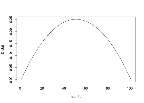
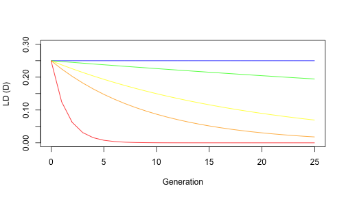
class: center, middle, inverse, title-slide

.title[
# Linkage disequilibrium
]
.author[
### Jinliang Yang
]
.date[
### Jan. 26, 2024
]

---

# Two SNP Loci

.pull-left[
<div align="center">
<img src="dogs.jpg" height=150>
</div>
]

.pull-right[
- dog 1: AA AA __TT__ CC __CC__ 
- dog 2: AA AA __CC__ CC __GG__
- dog 3: AA AA __CT__ CC __CC__ 
- dog 4: AA AA __CT__ CC __GC__
- dog 5: AA AA __CC__ CC __CC__
]

---------

.pull-right[
- dog 1: A A __T__ C __C__ / A A __T__ C __C__
- dog 2: A A __C__ C __G__ / A A __C__ C __G__
- dog 3: A A __C__ C __C__ / A A __T__ C __C__
- dog 4: A A __C__ C __G__ / A A __T__ C __C__
- dog 5: A A __C__ C __C__ / A A __C__ C __C__
]

### Haplotype Phasing:  
- Involves separating maternally and paternally inherited copies of each chromosome into haplotypes to get a complete picture of genetic variation.

---

# Two or more SNP loci

The __expected haplotype frequency__ = the product of the frequencies of the individual alleles that make up the haplotype

.pull-left[
<div align="center">
<img src="dogs.jpg" height=150>
</div>
]

#### Example:

- Two loci: A and B with alleles `\(A_1\)` (T) `\(A_2\)` (C) and `\(B_1\)` (G) `\(B_2\)` (C)

- Consider Haplotype `\(A_1B_2\)` ( __--T-C__ )

- Allele frequencies: `\(f_{A_1}=0.4\)` and `\(f_{B_2} = 0.7\)`

- Expected frequency of the haplotype = `\(f_{A_1} \times f_{B_2} = 0.4 \times 0.7 = 0.28\)`

- Observed haplotype freq = 4/10 = 0.4

---

# Linkage Equilibrium (LE)

If the observed haplotype frequency fits expectations under HWE, the alleles are inherited independent of one another

- They are in __Linkage Equilibrium__,

`\begin{align*}
f_{AB} & = p_Ap_B \\
f_{Ab} & = p_Ap_b = p_A(1-p_B) \\
f_{aB} & = p_ap_B = (1- p_A)p_B \\
p_{ab} & = p_ap_b = (1 - p_A)(1 - p_B) \\
\end{align*}`

- Otherwise, would be in __Linkage Disequilibrium__
 - Genotype frequencies are __not__ as expected with independent assortment (and HWE)

`\begin{align*}
f_{AB} & \ne p_Ap_B \\
f_{Ab} & \ne p_Ap_b = p_A(1-p_B) \\
f_{aB} & \ne p_ap_B = (1- p_A)p_B \\
p_{ab} & \ne p_ap_b = (1 - p_A)(1 - p_B) \\
\end{align*}`

---

# Linkage Disequilibrium (LD)

LD measures the extent to which alleles are associated

- The non-random association between alleles at two loci

### Why do we care?

- Linkage mapping

- Information regarding effective population size/inbreeding

- Can be leveraged to detect genome structural variation, i.e., inversion

---

# Linkage Disequilibrium (LD)

.pull-left[
<div align="center">
<img src="ld.png" width=300>
</div>
]

.pull-right[
- Allele at one locus is correlated with allele at 2nd locus

- Non-random association of alleles
]

---

# Measuring LD: `\(D\)` Statistics

`\(D\)` stat measures the deviation of haplotype frequencies from expected values based on allele frequencies.

`\begin{align*}
D_{AB} & = f_{AB} - p_Ap_B \\
\end{align*}`

- `\(f_{AB}\)` is the observed freq of AB haplotype

- `\(p_Ap_B\)` is the expected freq given allele freqs

- If `\(D = 0\)`, the alleles are inherited independently.

`\begin{align*}
D_{AB} & = D_{ab} \\
 & = -D_{Ab} = -D_{aB} 
\end{align*}`

---

# Measuring LD: `\(D\)` Statistics

`\begin{align*}
D_{AB} & = f_{AB} - p_Ap_B \\
\end{align*}`

------------

.pull-left[
<div align="center">
<img src="ld.png" width=300>
</div>
]

.pull-right[
Observed:
- `\(p_{AB} = 3/10 = 0.3\)`

Expected: 
- `\(p_A = 3/10 = 0.3\)`
- `\(p_B = 3/10 = 0.3\)`
- `\(p_Ap_B = 0.3 \times 0.3 = 0.09\)`

LD:
- `\(D_{AB} = 0.3 - 0.09 = 0.21\)`
]

`\(D_{AB} \ne 0\)`
- A and B alleles are observed together more often than expected
- These two alleles are in LD

---
# Summary of LD

| Gamete | AB   | Ab   | aB   | ab  |
| :-------: | : ------ : | :-------: | :-------: | :-------: | 
| Observed  | `\(f_{AB}\)`    | `\(f_{Ab}\)`    | `\(f_{aB}\)`     | `\(f_{ab}\)`     | 
|           |  `\(r\)`        |  `\(s\)`        |  `\(t\)`   |  `\(u\)`       |
| Expected (HWE)  | `\(p_Ap_B\)`   | `\(p_Aq_b\)`    | `\(q_ap_B\)`    | `\(q_aq_b\)`    | 
| Obs - Exp | `\(+D\)` | `\(-D\)` | `\(-D\)` | `\(+D\)` |

- `\(r\)` and `\(u\)`: coupling gametes (AB and ab)
- `\(s\)` and `\(t\)`: repulsion gametes (Ab and aB)

Here, we know:
`\begin{align*}
p_A & = f_{AB} + f_{Ab} \\
p_B & = f_{AB} + f_{aB} \\
\end{align*}`

And 
`\begin{align*}
D_{AB} & = f_{AB} - p_Ap_B \\
 & = f_{AB} - (f_{AB} + f_{Ab})(f_{AB} + f_{aB}) = r - (r + s)(r + t) \\
 &  = r - r^2 - rt -sr -st = r(1 -r - t -s) - st \\
 & = ru -st \\
\end{align*}`

---
# Summary of LD

- `\(r\)` and `\(u\)`: coupling gametes (AB and ab)
- `\(s\)` and `\(t\)`: repulsion gametes (Ab and aB)

----------

`\begin{align*}
D & =  ru -st \\
\end{align*}`

### D = coupling gametes - repulsion gametes

---

# Range of `\(D\)` through simulation

```r
fab <- seq(0, 1, by=0.01)
pa <- seq(0, 1, by=0.01)
pb <- seq(0, 1, by=0.01)
plot(fab - pa * pb, type ="l", ylab="D stat", xlab="hap frq")
```

![](week1_c3_files/figure-html/unnamed-chunk-4-1.png)
---

# Range of `\(D\)`

If all gametes are AB or ab (completely linked) and `\(P_A =P_B = 0.5\)`

`\begin{align*}
D_{AB} & =  f_{AB} - p_Ap_B = 0.5 - 0.5 \times 0.5 = 0.25 \\
D_{AB} & = -D_{Ab}
\end{align*}`

Therefore, __ `\(D\)` ranges from `\(-0.25\)` to `\(0.25\)`__

- In real life, this range is not usually maximized and can be determined by allele frequencies

- Due to dependence on allele frequencies, D cannot be compared between different sets of loci

---

# Measuring LD: `\(D'\)`

Richard Lewontin described how to normalize D for easier interpretation

`\begin{align*}
D' & =  \frac{D}{D_{max}}
\end{align*}`

------------------

`\(D_{max}\)` is the max value of the greatest possible LD for a given set of allele frequencies.

If `\(D > 0\)`,
`\begin{align*}
D_{max} & =  min(p_Aq_b, q_ap_B)
\end{align*}`

If `\(D < 0\)`,

`\begin{align*}
D_{max} & =  min(p_Ap_B, q_aq_b)
\end{align*}`

- `\(D'\)` therefore ranges from 0 to 1

- `\(D'\)` allows to be more informative in comparisons

---

# From our prior example

`\begin{align*}
D_{AB} & = f_{AB} - p_Ap_B \\
\end{align*}`

------------

.pull-left[
<div align="center">
<img src="ld.png" width=300>
</div>
]

.pull-right[
Observed:
- `\(p_{AB} = 3/10 = 0.3\)`

Expected: 
- `\(p_A = 3/10 = 0.3\)`
- `\(p_B = 3/10 = 0.3\)`
- `\(p_Ap_B = 0.3 \times 0.3 = 0.09\)`

LD:
- `\(D_{AB} = 0.3 - 0.09 = 0.21\)`
]

`\begin{align*}
D & > 0 \\
D_{max} & =  min(p_Aq_b, q_ap_B) \\
& = min(0.3 \times 0.7, 0.7 \times 0.3) = 0.21 \\
D' &= \frac{D}{D_{max}} = 1
\end{align*}`

---

# Alternatives to D

Hill and Robertson use `\(r^2\)`: correlation between two loci
- ranges from 0 to 1

`\begin{align*}
r^2 = \frac{D^2}{p_Aq_ap_Bq_b}
\end{align*}`

Because `\(r^2\)` considers allele frequency while `\(D'\)` uses frequency for normalization, `\(D'\)` can be high with low `\(r^2\)`

---

# Comparison of `\(D\)`, `\(D'\)` and `\(r^2\)`

> From [Gaut and Long 2003](https://academic.oup.com/plcell/article/15/7/1502/6010073). Plant Cell

---

# Interpreting LD

### The case when `\(D' = 1\)` is referred to as __Complete LD__

- In this case, there are at most 3 of the 4 possible haplotypes present in the populations.

- The intuition behind complete LD is that the two loci are not being separated by a recombination in this population since at least one of the haplotypes does not occur in the populations.

### The case when `\(r^2 = 1\)` is referred to as __Perfect LD__

- The case of perfect LD occurs when there are exactly 2 of the 4 possible haplotypes present in the population.

- As a result, the two loci also have the same allele frequencies.

- Loci that are in __perfect LD__ are necessarily in __complete LD__

---

# Causes of LD

- Natural selection

- Genetic drift

- Population subdivision/bottlenecks

- Inbreeding

### This does not only apply to haplotypes
- Alleles can be on different chromosomes and still in LD!

---

# Applications

- Mutation/gene mapping

- Detecting selection

- Estimating allele age

---

# LD decays over time via recombination

- `\(D_0\)` = LD at time zero
- `\(D_1\)` = LD at generation 1

The value of `\(D_1\)` depends on recombination rate

---

# Decay of LD

### Recombination frequency ( `\(c\)` )

The probability of crossover between A and B

- `\(c\)` ranges from 0 (no crossover) to 0.5 (independent loci)

For Example, we are interested in freq of `\(A_1B_1\)` haplotype in progeny

Two ways to get an `\(A_1B_1\)` gamete:

- #### From `\(A_1B_1/A_xB_x\)` with no recombination
  - Frequency of this `\(= r(1-c)\)`
  - `\(r\)` is frq of `\(p_{A_1B_1}\)` in parental gametes
  
--

- #### From recombination from `\(A_1B_x/A_xB_1\)` genotype
  - Frequency `\(=p_Ap_Bc\)`
  - `\(p_A = f_{A_1Bx}\)` and `\(p_B = f_{A_xB_1}\)`

---

# Frequency of `\(A_1B_1\)` in progeny

Frequency of the haplotype being maintained (no recombination) + frequency it is generated through recombination

`\begin{align*}
r_1 = r(1-c) + p_Ap_Bc
\end{align*}`

### What about LD in progeny?

Observed - expected:

`\begin{align*}
D_1 & = r_1 - p_Ap_B \\
\end{align*}`

Substitute in `\(r_1\)` from above,

`\begin{align*}
D_1 & = r(1-c) + p_Ap_Bc - p_Ap_B \\
& = r(1-c) - p_Ap_B(1-c) \\
& = (1-c)(r - p_Ap_B)
\end{align*}`

Note that `\(r\)` is the observed haplotype freq `\(f_{AB}\)`,

`\begin{align*}
D_1 & = D(1-c)
\end{align*}`

---

# LD after `\(t\)` generations

`\begin{align*}
D_t & = D(1-c)^t
\end{align*}`

For unlinked loci ( `\(c =0.5\)`, the red line), LD decays by half each generation.

```r
t = seq(0,25, by=1)
D <- function(t, c){return(0.25*(1-c)^t)} 
plot(t, D(t, c=0), type="l", col="blue", ylim=c(0, 0.3), xlab="Generation", ylab="LD (D)")
lines(t, D(t, c=0.01), type="l", col="green")
lines(t, D(t, c=0.05), type="l", col="yellow")
lines(t, D(t, c=0.1), type="l", col="orange")
lines(t, D(t, c=0.5), type="l", col="red")
```

![](week1_c3_files/figure-html/unnamed-chunk-5-1.png)