Rice data

Download the Rice Diversity Panel data RiceDiversity.44K.MSU6.Genotypes_PLINK.zip from http://ricediversity.org/data/sets/44kgwas/.

Genotypic data

rice <- read.table("http://www.ricediversity.org/data/sets/44kgwas/RiceDiversity_44K_Phenotypes_34traits_PLINK.txt", header=TRUE, stringsAsFactors = FALSE, sep = "\t")

rice <- rice[, 1:3]
set.seed(123579)
for(i in 1:1000){
   ## add a fake genotype assuming the pop in HWE
   p = runif(n=1, min=0.05, max=0.5)
   q = 1-p
   rice$geno <- sample(c(0,1,2), size=nrow(rice), prob=c(p^2, 2*p*q, q^2), replace=TRUE)
   names(rice)[ncol(rice)] <- paste0("m", i)
}

Check the genotype, i.e., the minor allele frequency

table(rice$m1)

## 
##   0   1   2 
##   4  61 348

a1 <- 4*2+61
a1/(2*nrow(rice)) #p

## [1] 0.08353511

Apply the method to all the markers:

# A function to calculate minor allele frequencies for all the markers
maf <- function(rice){
   df <- data.frame()
   for(i in 4:ncol(rice)){
      tb <- as.data.frame(table(rice[,i]))
      a1 <- 2*tb$Freq[1] + tb$Freq[2]
      frq <- data.frame(marker=names(rice)[i], maf=a1/(2*nrow(rice)))
      if(frq$maf > 0.5){
         frq$maf <- 1 - frq$maf
      }
      df <- rbind(df, frq)
   }
   return(df)
}
out <- maf(rice)

hist(out$maf, breaks=30, col="blue", xlim=c(0, 0.5), main="MAF distribution", xlab="freq")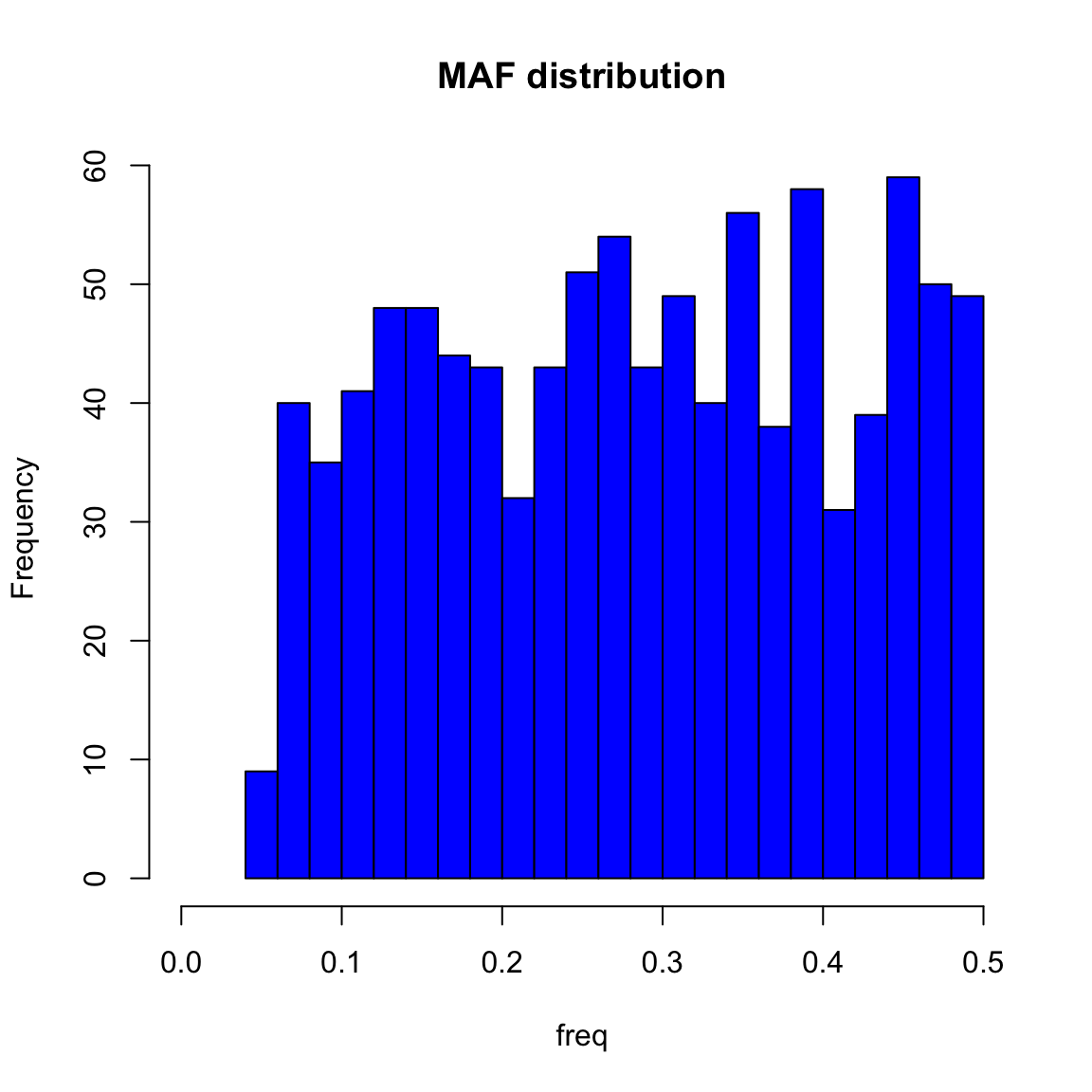

Phenotype data

Simulate QTLs controlling flowering time

Simulate phenotype using genotype data given number of QTLs and heritability.

sim_qtl_pheno <- function(geno, h2, nqtl){
#' @param geno genotype data, col1=genoid, col2 and after=snpid, coding: 0,1,2 (no missing data allowed) [data.frame].
#' @param h2 Broad sense heritability of the trait [numeric(0-1)].
#' @param nqtl number of QTL [interger].
#' @param distribution [character=norm]
#'
#' @return return A list of many values.
#'
#' @examples
#' geno <- read.table("data/geno.txt", header=TRUE)
#' pheno <- sim_qtl_pheno(geno, h2=0.7, alpha=0.5, nqtl=10, distribution="norm")
#' y <- pheno[['y']]
    X <- geno[, -1]
    n <- nrow(X)
    m <- ncol(X)
      
    set.seed(1237)
    #Sampling QTN
    QTN.position <- sample(m, nqtl, replace=F)
    SNPQ <- as.matrix(X[, QTN.position])

    message(sprintf("### [simpheno], read in [ %s ] SNPs for [ %s ] plants and simulated [ %s ] QTLs",
                    m, n, nqtl))

    #Simulate phenotype
    addeffect <- rnorm(nqtl,0,1)
    
    effect <- SNPQ%*%addeffect
    effectvar <- var(effect)
    residualvar <- (effectvar - h2*effectvar)/h2
    residual <- rnorm(n, 0, sqrt(residualvar))
    y <- effect + residual

    return(data.frame(y=y, SNPQ=SNPQ))
}

Apply the QTL simulation function to simulate phenotype with the given values of the h2 and number of QTLs nqtl.

set.seed(1237)
ph <- sim_qtl_pheno(geno=rice[, -2:-3], h2=0.9, nqtl=2)

## ### [simpheno], read in [ 1000 ] SNPs for [ 413 ] plants and simulated [ 2 ] QTLs

# assuming the values deviated from 100 days
ph$y <- ph$y+100
rice$Flowering.time.at.Arkansas <- ph$y
names(rice)[3] <- "ft"

Plot the phenotypic distribution:

# phenotypes
hist(rice$ft, breaks=30, col="blue", 
     main="Distribution of the flowering time values",
     xlab="flowering time (days)")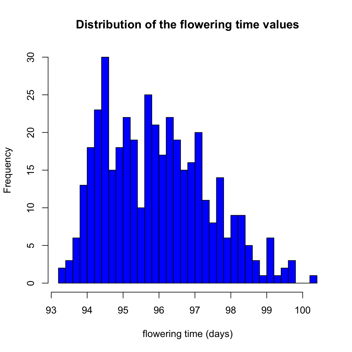

Average effect of the markers

\(Y = G + E\)

\(Y = \sum_{i=1}^n{G_i} + E\) for a population with \(i\) markers

\(G = A + D\)

If we find \(A_i\) for \(i\)th marker, then

\(\hat{Y} = \sum_{i=1}^n{A_i}\)

Single locus

gfunction <- function(a=1, d=0, p=1/2){
   # a: additive effect
   # d: dominant effect
   # p: allele frequency for the A1 allele
   
   q = 1-p
   # allele sub effect
   alpha <- a + d*(q-p)
   a1a1 <- 2*alpha*q
   a1a2 <- (q-p)*alpha
   a2a2 <- -2*p*alpha
   
   # population mean
   M <- a*(p-q) + 2*d*p*q
   # return a data.frame with genotype values and breeding values
   return(data.frame(N1=c(0,1,2), gv=c(-a-M,d-M,a-M), bv=c(a2a2, a1a2, a1a1)))
}

A1A1 -> 2
A1A2 -> 1
A2A2 -> 0

A1A1 <- mean(subset(rice, m1 == 2)$ft, na.rm=TRUE)
A1A2 <- mean(subset(rice, m1 == 1)$ft, na.rm=TRUE)
A2A2 <- mean(subset(rice, m1 == 0)$ft, na.rm=TRUE)

### mid point
m <- (A1A1 + A2A2)/2
a <- A1A1 - m
d <- A1A2 - m
df <- as.data.frame(table(rice$m1))
# allele freq for A1 (2 coding)
p <- (2*df[df$Var1==2,]$Freq + df[df$Var1==1,]$Freq)/(2*sum(df$Freq))

out <- gfunction(a=a, d=d, p=p)
avg <- (out$bv[1] - out$bv[3])/2

Next we wrap it into a function to calcuate the avg effect for all the markers

avgfun <- function(rice){
   
   outdf <- data.frame()
   for(i in 4:ncol(rice)){
      A1A1 <- mean(subset(rice, rice[,i] == 2)$ft, na.rm=TRUE)
      A1A2 <- mean(subset(rice, rice[,i] == 1)$ft, na.rm=TRUE)
      A2A2 <- mean(subset(rice, rice[,i] == 0)$ft, na.rm=TRUE)
      
      ### mid point
      m <- (A1A1 + A2A2)/2
      a <- A1A1 - m
      d <- A1A2 - m
      df <- as.data.frame(table(rice[,i]))
      # allele freq for A1 (2 coding)
      p <- (2*df[df$Var1==2,]$Freq + df[df$Var1==1,]$Freq)/(2*sum(df$Freq))

      out <- gfunction(a=a, d=d, p=p)
      avg <- (out$bv[1] - out$bv[3])/2
      
      tem <- data.frame(snp=names(rice)[i], eff=avg)
      outdf <- rbind(outdf, tem)
   }
   return(outdf)
}

outdf <- avgfun(rice)

plot(1:1000, abs(outdf$eff))

outdf$abseff <- abs(outdf$eff)
outdf <- outdf[order(outdf$abseff, decreasing = TRUE),]

Additive and dominance variance

Breeder’s equation

\[\begin{align*} R & = ih^2\sigma_P/L \\ & ih\sigma_A/L \\ \end{align*}\]

Because \(G = A + D\), then

\[\begin{align*} \sigma_G^2 & = \sigma_A^2 + \sigma_D^2 + 2\sigma_{A, D} \end{align*}\]

And \(\sigma_{A, D}=0\) in a HWE population, therefore,

\[\begin{align*} \sigma_G^2 & = \sigma_A^2 + \sigma_D^2 \end{align*}\]

Genotype	Freq	Breeding Value	\(A^2\)	Dominance Deviation	\(D^2\)
\(A_1A_1\)	\(p^2\)	\(2q\alpha\)	\((2q\alpha)^2\)	\(-2q^2d\)	\((-2q^2d)^2\)
\(A_1A_2\)	\(2pq\)	\((q-p)\alpha\)	\((q-p)^2\alpha^2\)	\(2pqd\)	\((2pqd)^2\)
\(A_2A_2\)	\(q^2\)	\(-2p\alpha\)	\((-2p\alpha)^2\)	\(-2p^2d\)	\((-2p^2d)^2\)

The additive and dominance genetic variance in a HWE population is:

\[\begin{align*} \sigma_A^2 & = 2pq(a + d(q-p))^2 \\ \sigma_D^2 & = (2pqd)^2 \\ \end{align*}\]

Write the Vg function

\[\begin{align*} \sigma_A^2 & = 2pq(a + d(q-p))^2 \\ \sigma_D^2 & = (2pqd)^2 \\ \end{align*}\]

vfun <- function(a=1, dod=0, p=seq(0,1, by=0.01)){
   # a: additive value, [num, =1]
   # dod: degree of dominance, [num, =0]
   # p: allele frequency of the A1 allele, [vector, =seq(0,1, by=0.01)]
   
   #a = 1
   d = dod*a #<< get the dominance value
   q = 1- p

   df <- data.frame(p=p, 
                    va=2*p*q*(a + d*(q-p))^2, 
                    vd=(2*p*q*d)^2)
   df$vg <- df$va + df$vd
   return(df)
}

Heritability calculation

h2fun <- function(rice){
   
   outdf <- data.frame()
   for(i in 4:ncol(rice)){
      A1A1 <- mean(subset(rice, rice[,i] == 2)$ft, na.rm=TRUE)
      A1A2 <- mean(subset(rice, rice[,i] == 1)$ft, na.rm=TRUE)
      A2A2 <- mean(subset(rice, rice[,i] == 0)$ft, na.rm=TRUE)
      
      ### mid point
      m <- (A1A1 + A2A2)/2
      a <- A1A1 - m
      d <- A1A2 - m
      df <- as.data.frame(table(rice[,i]))
      # allele freq for A1 (2 coding)
      p <- (2*df[df$Var1==2,]$Freq + df[df$Var1==1,]$Freq)/(2*sum(df$Freq))

      out <- vfun(a=a, dod=d/a, p=p)
      out$snp <- names(rice)[i]
      
      outdf <- rbind(outdf, out)
   }
   return(outdf)
}

outdf2 <- h2fun(rice)

plot(1:1000, abs(outdf2$vg), ylab="Variance explained by markers")

Broad sense heritability

\(H^2 = V_G / V_P\)

V <- subset(outdf2, snp %in% c("m329", "m983") )
Vg <- sum(V$vg, na.rm=T)
Vp <- var(rice$ft)
Vg/Vp

Narrow sense heritability

\(h^2 = V_A / V_P\)

Va <- sum(V$va, na.rm=T)
Va/Vp

Breeder’s equation

Intensity of selection ( \(i\) )

# function for selection intensity
ifun <- function(p=0.5){
  x=qnorm(p=(1-p)) # get the truncation point
  z=dnorm(x) # get z
  return(z/p) # get i
}
p <- seq(0.0001, 1, by=0.0001)
i <- ifun(p)
plot(p, i)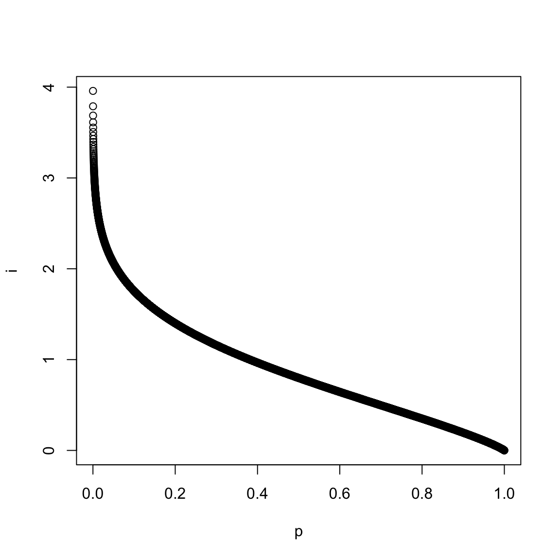

\[\begin{align*} R & = ih^2\sigma_P/L \\ & ih\sigma_A/L \\ \end{align*}\]

# response to selection
Rfun <- function(perc=0.05, h2, va){
   i <- ifun(p=perc)
   h <- sqrt(h2)
   return(i*h*sqrt(va))
}
   
outR <- Rfun(perc=0.05, h2=0.9, va=2.327923)

50/outR

## [1] 16.74656

A sib analysis

A swine breeder collected a set of data from a sib design: - 2 sires + 34 dams
- Each pair of parents has four offspring
- Measured body weight of the newborns

Calculate the estimate of heritability
Comment on any possible bias in the estimated heritability

Read in data

df <- read.csv("https://jyanglab.com/AGRO-931/data/swine_sib.csv")

Get the ANOVA table

\(Y = S + D + E\)

\(V_P = V_S + V_D + V_E\)

fit <- lm(weight ~ sire + dam, data=df)
summary(aov(fit))

##              Df Sum Sq Mean Sq F value   Pr(>F)    
## sire          1   6331    6331  17.978 3.73e-05 ***
## dam          33  24216     734   2.084  0.00141 ** 
## Residuals   163  57405     352                     
## ---
## Signif. codes:  0 '***' 0.001 '**' 0.01 '*' 0.05 '.' 0.1 ' ' 1

Variance components in a sib design

Source	df	Sums of Squares	MS	E(MS)
Sires	s-1	\(dn\sum\limits_{i=1}^s(\bar{p}_i - \bar{p})^2\)	\(MS_s\)	\(= \sigma_w^2 + n\sigma_d^2 + dn\sigma_s^2\)
Dams (Sires)	s(d-1)	\(n\sum\limits_{i=1}^s\sum\limits_{j=1}^d(\bar{p}_{ij} - \bar{p}_i)^2\)	\(MS_d\)	\(= \sigma_w^2 + n\sigma_d^2\)
Sibs (Dams)	sd(n-1)	\(\sum\limits_{i=1}^s\sum\limits_{j=1}^d\sum\limits_{k=1}^n(p_{ijk} - \bar{p}_{ij})^2\)	\(MS_w\)	\(= \sigma_w^2\)

vw <- 352
n=4 # number of kids per full-sib family
vd <- (734 - vw)/n 
d=33
vs <- (6331 - 734)/(d*n)

vp <- vd + vs + vw

Summary of the variance components

A key concept in the ANOVA is that the variance between-family (group) is equal to the covariance within-family (group).

Observational	Covariance and causal components	estimated values
Sires	\(\sigma_s^2 = Cov(HS)\)	\(=\frac{1}{4}\sigma_A^2\)
Dams	\(\sigma_d^2 = Cov(FS) - Cov(HS)\)	\(=\frac{1}{4}\sigma_A^2 + \frac{1}{4}\sigma_D^2\)
Progeny	\(\sigma_w^2 = V_P - Cov(FS)\)	\(= \frac{1}{2}\sigma_A^2 +\frac{3}{4}\sigma_D^2\)
Total	\(\sigma_T^2 = V_P = \sigma_s^2 + \sigma_d^2 + \sigma_w^2\)	\(=\sigma_A^2 + \sigma_D^2 + \sigma_E^2\)
Sires + Dams	\(\sigma_s^2 + \sigma_d^2 = Cov(FS)\)	\(=\frac{1}{2}\sigma_A^2 + \frac{1}{4}\sigma_D^2\)

\(\sigma_s^2 = Cov(HS) = 1/4 \sigma_A^2\)

va <- 4*vs

\(h^2 = V_A/V_P\)

va/vp

## [1] 0.3462044

\(\sigma_d^2 = Cov(FS) - Cov(HS) = 1/4 \sigma_A^2 + 1/4 \sigma_D^2\)

Vd = 4*vd  - va

Lab4: Summary

Jinliang Yang

Nov. 16, 2020

Rice data

Genotypic data

Phenotype data

Simulate QTLs controlling flowering time

Average effect of the markers

Single locus

Additive and dominance variance

Breeder’s equation

Write the Vg function

Heritability calculation

Breeder’s equation

Intensity of selection ( \(i\) )

A sib analysis

Read in data

Get the ANOVA table

Variance components in a sib design

Summary of the variance components