Additive and dominance variance
Single locus
Because \(G = A + D\), then
\[\begin{align*} \sigma_G^2 & = \sigma_A^2 + \sigma_D^2 + 2\sigma_{A, D} \end{align*}\]
And \(\sigma_{A, D}=0\) in a HWE population, therefore,
\[\begin{align*} \sigma_G^2 & = \sigma_A^2 + \sigma_D^2 \end{align*}\]
| Genotype | Freq | Breeding Value | \(A^2\) | Dominance Deviation | \(D^2\) | |
|---|---|---|---|---|---|---|
| \(A_1A_1\) | \(p^2\) | \(2q\alpha\) | \((2q\alpha)^2\) | \(-2q^2d\) | \((-2q^2d)^2\) | |
| \(A_1A_2\) | \(2pq\) | \((q-p)\alpha\) | \((q-p)^2\alpha^2\) | \(2pqd\) | \((2pqd)^2\) | |
| \(A_2A_2\) | \(q^2\) | \(-2p\alpha\) | \((-2p\alpha)^2\) | \(-2p^2d\) | \((-2p^2d)^2\) |
The additive and dominance genetic variance in a HWE population is:
\[\begin{align*} \sigma_A^2 & = 2pq(a + d(q-p))^2 \\ \sigma_D^2 & = (2pqd)^2 \\ \end{align*}\]
Graphic representation of Va, Vd, and Vg
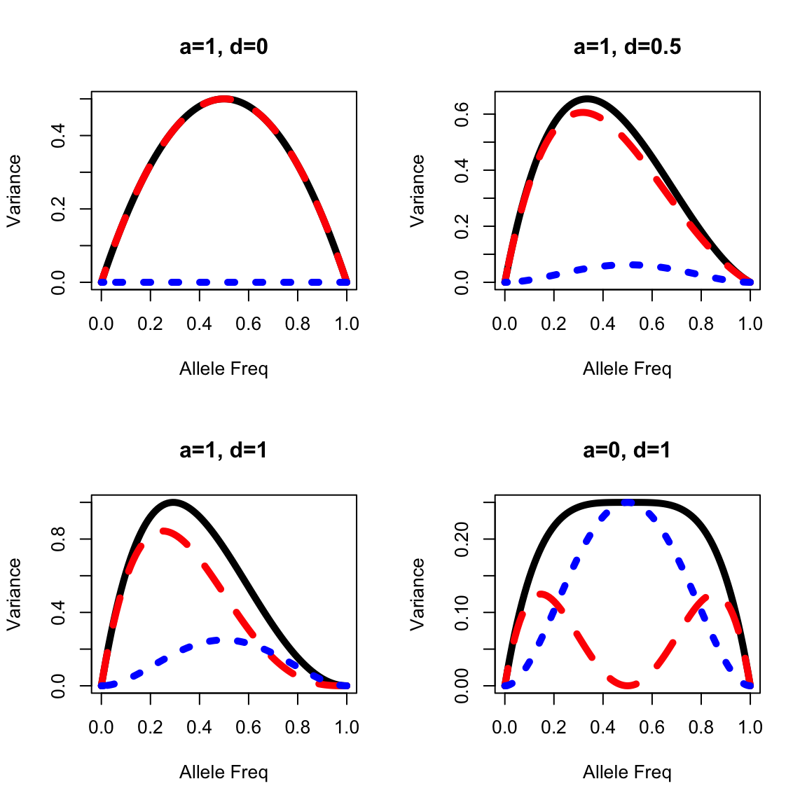
- Genetic variance components are typically maximized at intermediate allele frequencies.
- Additive genetic variance typically makes up most of the genetic variance except in unusual situations, such as when overdominant gene action is present or allele frequencies are at the extremes.
Write the Vg function
\[\begin{align*} \sigma_A^2 & = 2pq(a + d(q-p))^2 \\ \sigma_D^2 & = (2pqd)^2 \\ \end{align*}\]
vfun <- function(a=1, dod=0, p=seq(0,1, by=0.01)){
   # a: additive value, [num, =1]
   # dod: degree of dominance, [num, =0]
   # p: allele frequency of the A1 allele, [vector, =seq(0,1, by=0.01)]

   #a = 1
   d = dod*a #<< get the dominance value
   q = 1- p

   df <- data.frame(p=p,
                    va=2*p*q*(a + d*(q-p))^2,
                    vd=(2*p*q*d)^2)
   df$vg <- df$va + df$vd
   return(df)
}
Apply the function for the pure additive locus
out <- vfun(a=1, dod=0, p=seq(0,1, by=0.01))

plot(out$p, out$vg, lty=1, lwd=5, type="l", xlab="Allele Freq", ylab="Variance", main="a=1, dod=0")
lines(out$p, out$va, lty=2, lwd=5, col="red")
lines(out$p, out$vd, lty=3, lwd=5, col="blue")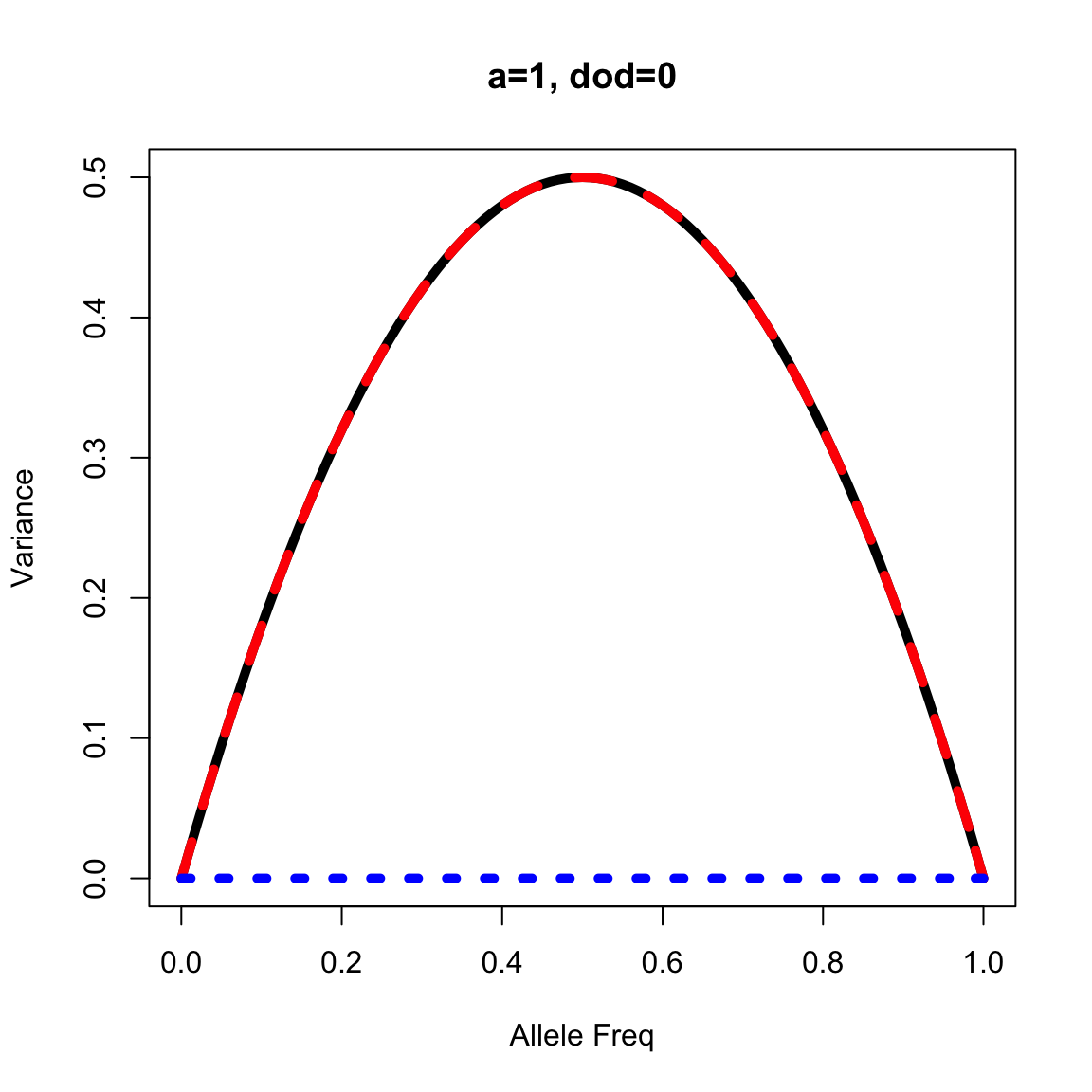
Incomplete dominance (or partial dominance)
out <- vfun(a=1, dod=0.5, p=seq(0,1, by=0.01))

plot(out$p, out$vg, lty=1, lwd=5, type="l", xlab="Allele Freq", ylab="Variance", main="a=1, dod=0.5")
lines(out$p, out$va, lty=2, lwd=5, col="red")
lines(out$p, out$vd, lty=3, lwd=5, col="blue")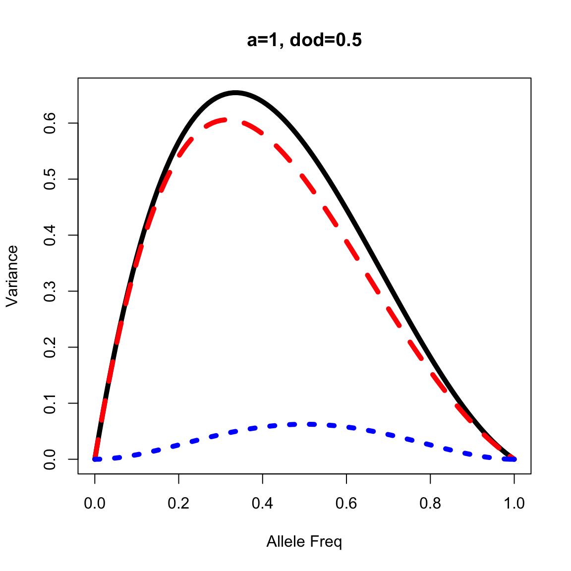
Complete dominance
out <- vfun(a=1, dod=1, p=seq(0,1, by=0.01))

plot(out$p, out$vg, lty=1, lwd=5, type="l", xlab="Allele Freq", ylab="Variance", main="a=1, dod=1")
lines(out$p, out$va, lty=2, lwd=5, col="red")
lines(out$p, out$vd, lty=3, lwd=5, col="blue")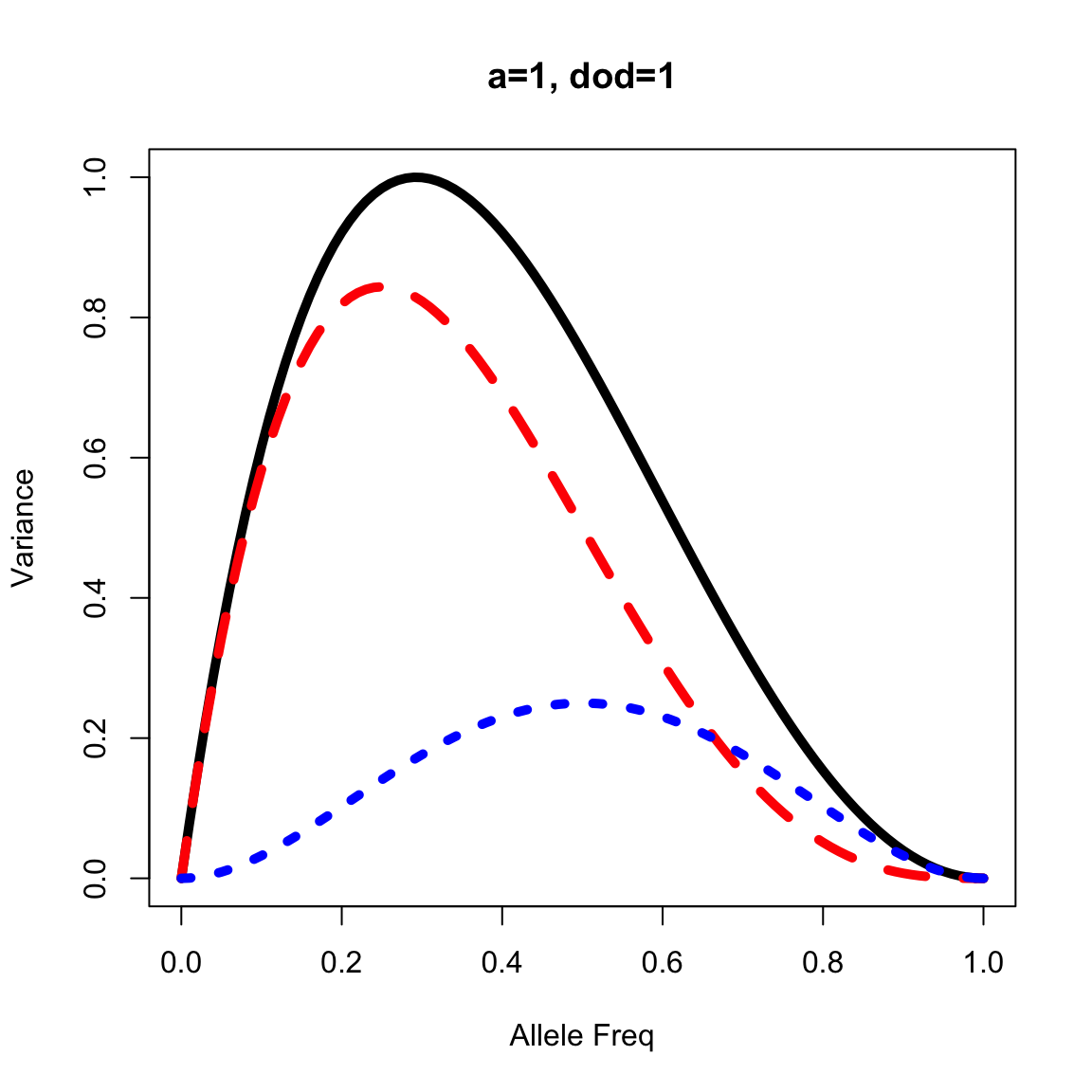
Let’s find out at what allele freq that gives Vd > Va
##        p         va         vd         vg
## 68  0.67 0.19262232 0.19554084 0.38816316
## 69  0.68 0.17825792 0.18939904 0.36765696
## 70  0.69 0.16444632 0.18301284 0.34745916
## 71  0.70 0.15120000 0.17640000 0.32760000
## 72  0.71 0.13852952 0.16957924 0.30810876
## 73  0.72 0.12644352 0.16257024 0.28901376
## 74  0.73 0.11494872 0.15539364 0.27034236
## 75  0.74 0.10404992 0.14807104 0.25212096
## 76  0.75 0.09375000 0.14062500 0.23437500
## 77  0.76 0.08404992 0.13307904 0.21712896
## 78  0.77 0.07494872 0.12545764 0.20040636
## 79  0.78 0.06644352 0.11778624 0.18422976
## 80  0.79 0.05852952 0.11009124 0.16862076
## 81  0.80 0.05120000 0.10240000 0.15360000
## 82  0.81 0.04444632 0.09474084 0.13918716
## 83  0.82 0.03825792 0.08714304 0.12540096
## 84  0.83 0.03262232 0.07963684 0.11225916
## 85  0.84 0.02752512 0.07225344 0.09977856
## 86  0.85 0.02295000 0.06502500 0.08797500
## 87  0.86 0.01887872 0.05798464 0.07686336
## 88  0.87 0.01529112 0.05116644 0.06645756
## 89  0.88 0.01216512 0.04460544 0.05677056
## 90  0.89 0.00947672 0.03833764 0.04781436
## 91  0.90 0.00720000 0.03240000 0.03960000
## 92  0.91 0.00530712 0.02683044 0.03213756
## 93  0.92 0.00376832 0.02166784 0.02543616
## 94  0.93 0.00255192 0.01695204 0.01950396
## 95  0.94 0.00162432 0.01272384 0.01434816
## 96  0.95 0.00095000 0.00902500 0.00997500
## 97  0.96 0.00049152 0.00589824 0.00638976
## 98  0.97 0.00020952 0.00338724 0.00359676
## 99  0.98 0.00006272 0.00153664 0.00159936
## 100 0.99 0.00000792 0.00039204 0.00039996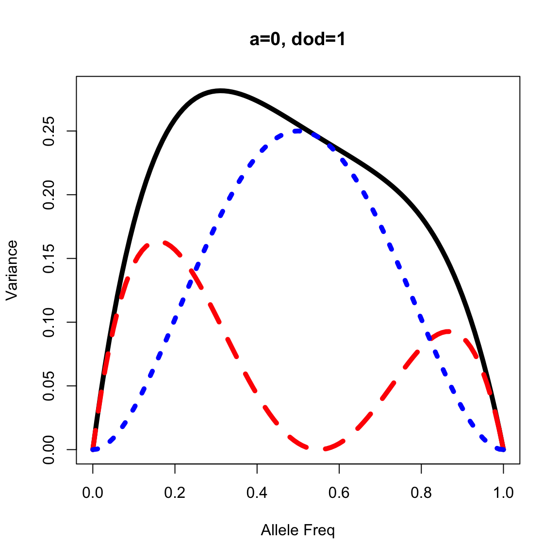
Rice data
Download the Rice Diversity Panel data RiceDiversity.44K.MSU6.Genotypes_PLINK.zip from http://ricediversity.org/data/sets/44kgwas/.
Phenotype data
We will use the read.table function to read the phenotype file RiceDiversity_44K_Phenotypes_34traits_PLINK.txt from here.
# phenotypes
rice <- read.table("http://www.ricediversity.org/data/sets/44kgwas/RiceDiversity_44K_Phenotypes_34traits_PLINK.txt", header=TRUE, stringsAsFactors = FALSE, sep = "\t")

rice <- rice[, 1:3]

## add a fake genotype assuming the pop in HWE
p = 0.2
q = 1-p
rice$geno <- sample(c(0,1,2), size=nrow(rice), prob=c(p^2, 2*p*q, q^2), replace=TRUE)
Let’s find out the genotypic value and breeding value for each individual.
Step1: find out \(a, d, -a\), and \(M\)
The number of copies of the A1 allele:
- A1A1 -> 2
- A1A2 -> 1
- A2A2 -> 0
A1A1 <- mean(subset(rice, geno == 2)$Flowering.time.at.Arkansas, na.rm=TRUE)
A1A2 <- mean(subset(rice, geno == 1)$Flowering.time.at.Arkansas, na.rm=TRUE)
A2A2 <- mean(subset(rice, geno == 0)$Flowering.time.at.Arkansas, na.rm=TRUE)

### mid point
m <- (A1A1 + A2A2)/2
a <- A1A1 - m
d <- A1A2 - m

### Population mean
M1 <- mean(rice$Flowering.time.at.Arkansas, na.rm=T)

### M = a*(p-q) + 2*d*p*q
df <- as.data.frame(table(rice$geno))
# allele freq for A1 (2 coding)
p <- (2*df[df$Var1==2,]$Freq + df[df$Var1==1,]$Freq)/(2*sum(df$Freq))
q <- 1-p
M2 <- a*(p-q) + 2*d*p*q
M2 <- M2 +m
A simple function to calculate genotypic values
gfun <- function(a=1, d=0, p=1/2){
   # a: additive effect
   # d: dominance effect
   # p: allele frequency for the A1 allele

   q = 1-p
   # allele sub effect
   alpha <- a + d*(q-p)
   a1a1 <- 2*alpha*q
   a1a2 <- (q-p)*alpha
   a2a2 <- -2*p*alpha

   # population mean
   M <- a*(p-q) + 2*d*p*q
   # return a data.frame with genotype values and breeding values
   return(data.frame(N1=c(0,1,2), gv=c(-a-M,d-M,a-M), bv=c(a2a2, a1a2, a1a1)))
}
Apply the function
##   N1         gv         bv         dd
## 1  0 -0.2222222 -0.4444444  0.2222222
## 2  1 -0.2222222  0.2222222 -0.4444444
## 3  2  1.7777778  0.8888889  0.8888889
Step2: Average effect for A1 and A2
Simulate a QTL
Simulate phenotype using genotype data given number of QTLs and heritability.
sim_qtl_pheno <- function(geno, h2, nqtl){
#' @param geno genotype data, col1=genoid, col2 and after=snpid, coding: 0,1,2 (no missing data allowed) [data.frame].
#' @param h2 Broad sense heritability of the trait [numeric(0-1)].
#' @param nqtl number of QTL [interger].
#' @param distribution [character=norm]
#'
#' @return return A list of many values.
#'
#' @examples
#' geno <- read.table("data/geno.txt", header=TRUE)
#' pheno <- sim_qtl_pheno(geno, h2=0.7, alpha=0.5, nqtl=10, distribution="norm")
#' y <- pheno[['y']]
    X <- geno[, -1]
    n <- nrow(X)
    m <- ncol(X)

    set.seed(1237)
    #Sampling QTN
    QTN.position <- sample(m, nqtl, replace=F)
    SNPQ <- as.matrix(X[, QTN.position])

    message(sprintf("### [simpheno], read in [ %s ] SNPs for [ %s ] plants and simulated [ %s ] QTLs",
                    m, n, nqtl))

    #Simulate phenotype
    addeffect <- rnorm(nqtl,0,1)

    effect <- SNPQ%*%addeffect
    effectvar <- var(effect)
    residualvar <- (effectvar - h2*effectvar)/h2
    residual <- rnorm(n, 0, sqrt(residualvar))
    y <- effect + residual

    return(data.frame(y=y, SNPQ=SNPQ))
}
Read in the genotypic data
## add a fake genotype assuming the pop in HWE
p = 0.5
q = 1-p
rice$geno2 <- sample(c(0,1,2), size=nrow(rice), prob=c(p^2, 2*p*q, q^2), replace=TRUE)

pout <- sim_qtl_pheno(geno=rice[, c("HybID", "geno", "geno2")], h2=0.31, nqtl=1)
## ### [simpheno], read in [ 2 ] SNPs for [ 413 ] plants and simulated [ 1 ] QTLsdf <- pout
vp <- var(df$y)
A1A1 <- mean(subset(df, SNPQ == 2)$y, na.rm=TRUE)
A1A2 <- mean(subset(df, SNPQ == 1)$y, na.rm=TRUE)
A2A2 <- mean(subset(df, SNPQ == 0)$y, na.rm=TRUE)
### mid point
m <- (A1A1 + A2A2)/2
a <- A1A1 - m
d <- A1A2 - m
out2 <- gfun(a=a, d=d, p=p)
out3 <- vfun(a=a, dod=d/a, p=p)
H2 <- out3$vg/vp
h2 <- out3$va/vp
h2## [1] 0.3479123