A maize experiment
A set of maize hybrids (N=345) crossed from male lines (M1, M2, M3, M4 and M5) and female lines (F1, F2, F3, F4, F5, F6).
The hybrids were planted in four environments, each with three replication.
Read in data
##   Male Female    ENV REP       Yld Moist  IVTD
## 1   M1     F1 2005_1   1 12.132546 11.80 70.01
## 2   M1     F1 2006_1   1  9.809719 11.16 70.48
## 3   M2     F1 2005_1   1  9.915348 11.70 69.71
## 4   M2     F1 2006_1   1 13.892623 11.10 67.07
## 5   M3     F1 2006_1   1  8.189426 11.60 70.46
## 6   M4     F1 2005_1   1 10.351882 11.50 69.67
Across environments
To learn about how to do data visulization and other in R.
Many other R statistics resources
## Warning: package 'ggplot2' was built under R version 3.4.4corn$geno <- paste(corn$Male, corn$Female, sep="x")
fsize=18
p1 <- ggplot(data=corn, aes(x=REP, y=Yld, fill= as.factor(REP)) ) +
geom_violin() +
facet_wrap(~ ENV) +
#guides(fill=FALSE) + factor(trait, levels=out$trait)
labs(y=NULL, fill="Rep") +
xlab("") +
ylab("") +
theme_bw() +
theme(axis.text.x=element_blank(), axis.ticks.x=element_blank(),
axis.text=element_text(size=fsize),
axis.title=element_text(size=fsize, face="bold"),
legend.title = element_text(size=fsize, face="bold"),
legend.text = element_text(size=fsize))
p1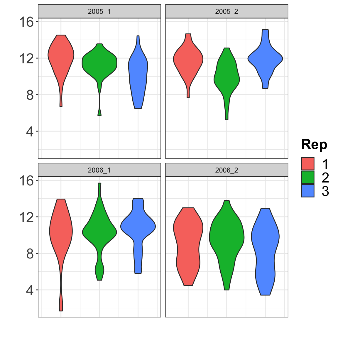
Half-sibs
One parent in common.
hs1 <- subset(corn, Male %in% c("M1", "M2"))

fit <- lm(Yld ~ Male + ENV + ENV:REP, data=hs1)
summary(aov(fit))
## Df Sum Sq Mean Sq F value Pr(>F)
## Male 1 1.9 1.925 0.594 0.44232
## ENV 3 38.6 12.876 3.972 0.00949 **
## ENV:REP 4 25.0 6.238 1.925 0.10994
## Residuals 134 434.4 3.241
## ---
## Signif. codes: 0 '***' 0.001 '**' 0.01 '*' 0.05 '.' 0.1 ' ' 1What is the among-families and within-families variance?
The intraclass correlation is 1.9/(1.9 + 3.2)
The covariance between two individuals
The covariance between two individuals in the same group is equal to the variance between groups.
Cov(HS) = Var(between)
Full-sibs
Both parents in common.
##     Male Female    ENV REP       Yld Moist  IVTD  geno
## 1     M1     F1 2005_1   1 12.132546 11.80 70.01 M1xF1
## 2     M1     F1 2006_1   1  9.809719 11.16 70.48 M1xF1
## 12    M2     F2 2005_1   1 11.719874 11.80 72.24 M2xF2
## 13    M2     F2 2006_1   1 12.642069 11.70 67.30 M2xF2
## 58    M1     F1 2005_1   2 11.911893 11.60 71.33 M1xF1
## 59    M1     F1 2006_1   2 11.358482 11.40 67.92 M1xF1
## 71    M2     F2 2005_1   2 12.283671 11.90 71.18 M2xF2
## 72    M2     F2 2006_1   2  9.480686 11.90 65.50 M2xF2
## 116   M1     F1 2005_1   3  9.243844 11.80 71.04 M1xF1
## 117   M1     F1 2006_1   3 12.021751 11.40 70.10 M1xF1
## 128   M2     F2 2005_1   3  8.370777 12.30 68.33 M2xF2
## 129   M2     F2 2006_1   3 11.389737 11.80 67.83 M2xF2
## 172   M1     F1 2005_2   1 12.338039 12.10 71.37 M1xF1
## 173   M1     F1 2006_2   1 12.096800  9.60 64.92 M1xF1
## 184   M2     F2 2005_2   1 10.505628 11.60 67.45 M2xF2
## 185   M2     F2 2006_2   1  7.315236  9.10 65.67 M2xF2
## 230   M1     F1 2005_2   2 13.108079 11.90 65.39 M1xF1
## 231   M1     F1 2006_2   2 12.052070  9.30 64.85 M1xF1
## 242   M2     F2 2005_2   2 10.316791 11.80 66.76 M2xF2
## 243   M2     F2 2006_2   2 10.184848  9.30 61.35 M2xF2
## 288   M1     F1 2005_2   3 11.831043 12.20 68.05 M1xF1
## 289   M1     F1 2006_2   3  8.080784  9.10 65.01 M1xF1
## 300   M2     F2 2005_2   3  8.675930 11.70 65.54 M2xF2
## 301 M2 F2 2006_2 3 8.259983 9.00 64.05 M2xF2## Df Sum Sq Mean Sq F value Pr(>F)
## geno 1 9.18 9.176 4.061 0.0622 .
## ENV 3 8.93 2.976 1.317 0.3056
## ENV:REP 4 13.68 3.420 1.514 0.2482
## Residuals 15 33.89 2.259
## ---
## Signif. codes: 0 '***' 0.001 '**' 0.01 '*' 0.05 '.' 0.1 ' ' 1Again, Cov(FS) = var(between)
Variance Components
corn$REP <- as.factor(corn$REP)

fit <- lm(Yld ~ Male + Female +  ENV + ENV:REP, data=corn)

##Perform simple ANOVA
aovResult <- aov(fit)


##Extract table of mean squares
summary(aovResult)[[1]]
## Df Sum Sq Mean Sq F value Pr(>F)
## Male 4 59.86 14.964 3.7421 0.005418 **
## Female 5 81.26 16.251 4.0641 0.001363 **
## ENV 3 285.33 95.112 23.7851 6.147e-14 ***
## ENV:REP 8 133.76 16.720 4.1813 8.843e-05 ***
## Residuals 324 1295.61 3.999
## ---
## Signif. codes: 0 '***' 0.001 '**' 0.01 '*' 0.05 '.' 0.1 ' ' 1