Data Types in R
For more information, please refer to Quick-R.
R has a wide variety of data types including scalars, vectors (numerical, character, logical), matrices, data frames, and lists.
Vectors
a <- c(1, 2, 5.3, 6, -2) # numeric vector
b <- c("one","two","three", "four", "five") # character vector
c <- c(TRUE,TRUE,TRUE,FALSE,TRUE) #logical vector
Refer to elements of a vector using subscripts.
## [1] 2 6Data Frames
In a data frame, different columns can have different modes (numeric, character, factor, etc.). This is similar to SAS and SPSS datasets.
##      ID Value Passed
## 1   one   1.0   TRUE
## 2   two   2.0   TRUE
## 3 three   5.3   TRUE
## 4  four   6.0  FALSE
## 5  five  -2.0   TRUE
Operators in R
Arithmetic Operators include:
| Operator | Description |
|---|---|
| + | addition |
| - | subtraction |
| * | multiplication |
| / | division |
| ^ or ** | exponentiation |
Logical Operators include:
| Operator | Description |
|---|---|
| > | greater than |
| >= | greater than or equal to |
| == | exactly equal to |
| != | not equal to |
R for Loop
Loops are used in programming to repeat a specific block of code.
Syntax of for loop
Example: for loop
Below is an example to count the number of even numbers in a vector.
x <- c(2,5,3,9,8,11,6)
count <- 0
for (i in 1:length(x)) {
  if(x[i] %% 2 == 0) {
    count = count + 1
    }
}
print(count)
## [1] 3The Central Limit Theorem (CLT)
- The CLT states that the sums of a set of random variables \((X_1, X_2, X_3, ..., X_n)\) is normally distributed no matter the distribution the individual X’s were sampled from, as long as they were sampled from identical distributions.
A simulation experiment
\[\begin{align*} Y_{i} = \sum\limits_{j=1}^{j=m} X_{ij} \alpha_{j} + \epsilon_i \end{align*}\]
- For a given individual ( \(i=1\) ) with a number of loci ( \(m=1,000\) )
- Each allele is \(X_j \in (A, a)\) , with the probability of \(p\) or \(1-p\)
- The effect of \(j\)th allele ( \(\alpha_j\) ) can be samples from any distribution (e.g., uniform distribution)
According to the CLT, if \(m\) is sufficiently large, the sum is normally distributed.
Simulate one dividual
Simulate an individual’s phenotypic value. In this individual, the phenotype is determined by m number of markers with marker freq = 0.5. The markers’ effects ( \(\alpha\) ) are randomly draws from a uniform distribution.
m <- 1000
## for each allele, the chance of A or a is equal to 0.5
x <- rbinom(n=m, size=1, prob=0.5)
## sample effect from a uniform distribution:
a <- runif(n=m)
y <- sum(x*a) + 0
y
## [1] 250.1851Apply the above procedure to a population composed of n individuals.
set.seed(1234) # seed for random number generator
m <- 1000
n <- 2000 # simulate a population of 2,000 individuals
out <- c() # create an empty vector
for(i in 1:n){ #<<
  x <- rbinom(m, size=1, prob=0.5) ## for each allele, the chance of A = 0.5
  a <- runif(m) ## sample effect from a uniform distribution:
  y <- sum(x*a)
  out <- c(out, y)
}
Plot the result
#shapiro.test(out) # W = 0.99928, p-value = 0.6622
hist(out, breaks=50, col="#b8860b", main="Phenotype Distribution", xlab="")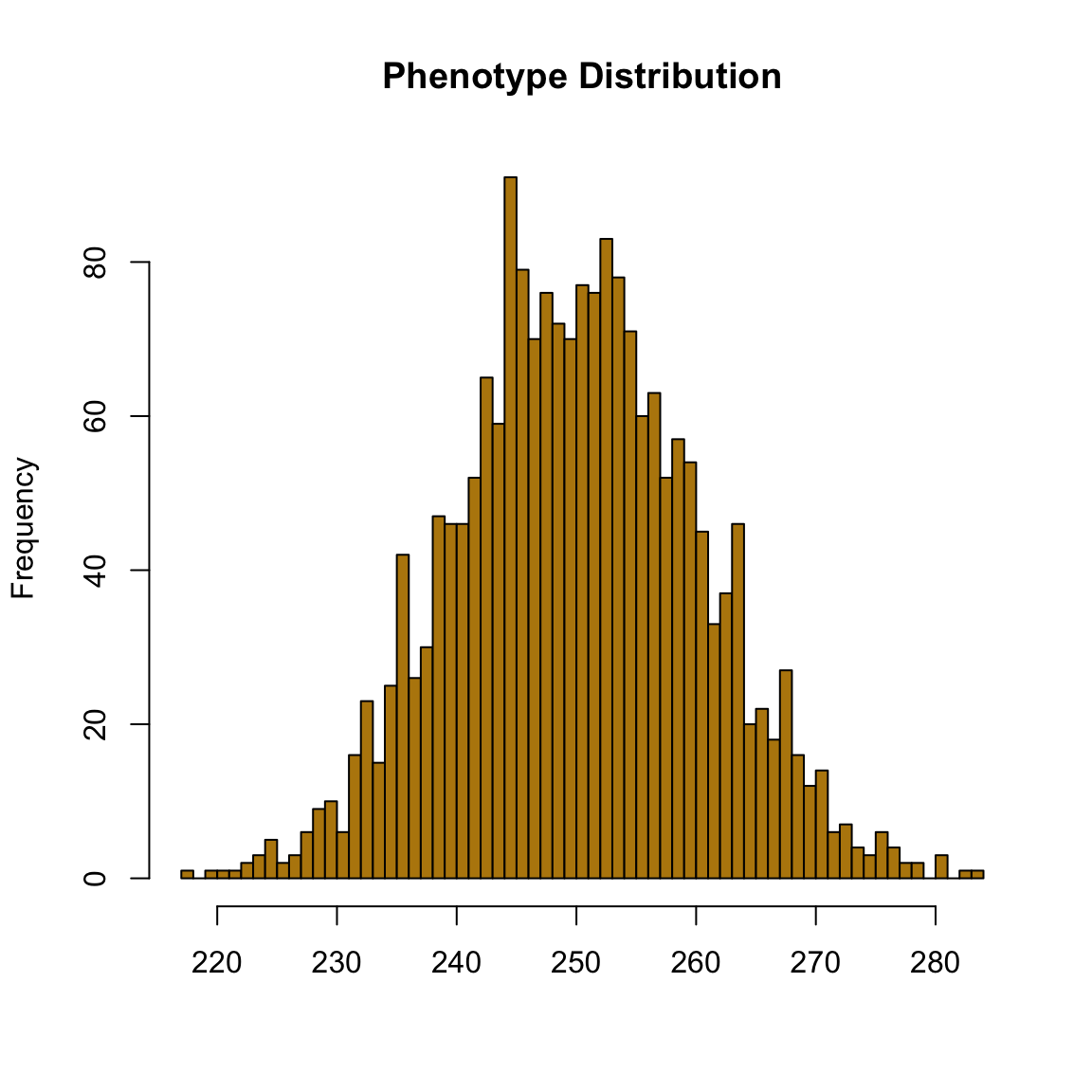
Determine what does the sufficiently large mean?
Pack the abvoe simulation procedure into an R function:
sim_clt <- function(m=1, n=2000){
  # m: number of markers, m=1
  # n: number of individuals, n=2000
  out <- c() # create an empty vector
  for(i in 1:n){ #<<
    x <- rbinom(m, size=1, prob=0.5) ## for each allele, the chance of A = 0.5
    a <- runif(m) ## sample effect from a uniform distribution:
    y <- sum(x*a)
    out <- c(out, y)
  }
  # output p.value
  return(shapiro.test(out)$p.value)
}
Then apply the function using an R for loop:
We will run a sequene of number of markers from 10 to 1000, with the increment of 10.
set.seed(12345)
pval <- c() # create an empty vector as the output
#
num <- seq(from =10, to =1000, by=10) #
for(i in num){
  # here we apply the function for the situation with i markers
  tem <- sim_clt(m=i, n=2000)
  pval <- c(pval, tem)
}
Again, let’s plot the result!
plot(x=num, y=-log10(pval), col="#b8860b", main="Phenotype Distribution", xlab="")
abline(h=-log10(0.01))